If you have ever lived in a suburban neighborhood or out in the farmlands, you likely have noticed a whitetail deer or two roaming around during an autumn evening. It doesn’t really catch you off guard; after all, it’s a deer and deer are everywhere. A year later, you look out your living room window and see four or five deer, the next autumn there are 10, and the next, 15. What’s going on? Where are all these deer coming from? Well, the answer has to do with what biologists refer to as population growth curves.
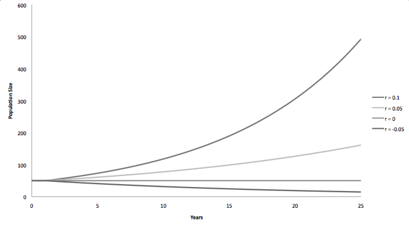
Wildlife biologists have determined that there are two different types of growth curves that the majority of wildlife follows. The first is called “exponential growth,” which relies on the basic principles of population dynamics: birth, death, immigration, and emigration. Biologists can use these four values to calculate the annual rate of change for the population, enabling them to predict the future population size of the future.
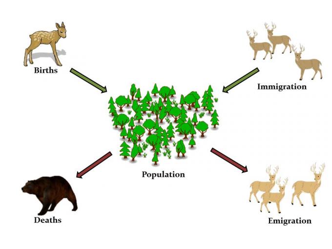
Rate of change (r) = Birth – Death + Immigration – Emigration
Small differences in the rate of change can result in very different outcomes for a population. For example, if a deer population started with 50 individuals and increases annually by ten percent (r = 0.1), the population would double in eight years. Whereas, if the population increased by only five percent (r = 0.05) each year, it would take 15 years to double.
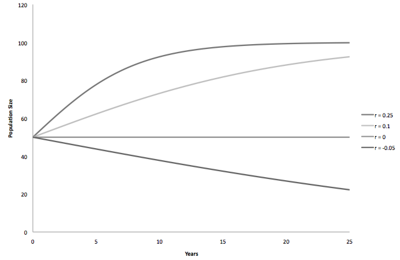
One of the flaws of the exponential growth curve is that it assumes there is no population ceiling. Resources that wildlife rely on (food, habitat, and water) are all finite and can be exhausted if the population grows too large. To address the fact there is a limit to population growth, known as carrying capacity; biologists use what is known as a “logistic curve,” In this case, our carrying capacity is limiting the population to 100 individuals. At higher population growth rates (0.25 and 0.01), the population begins to flatten out as it reaches 100. The rate of growth actually decreases as a population reaches carrying capacity.
You may have heard news last week that federal wildlife managers intend to delist the Yellowstone population of grizzly bears. They cited carrying capacity in their argument, which is a pretty good real-world case of the logistic curve described here. The habitat is full, so the amplitude of population swings is decreased over time.
When a population tends to grow in an exponential manner, it’s known as “density-independence.” The number of individuals in the population doesn’t affect the growth rate, it remains constant. By including carrying capacity and an upper population limit, the growth rate changes as population increase, this is known as a “density-dependent” relationship. In this case the wildlife population growth is dependent on other environmental factors.
It is important to note that these projections occur in what is called a “closed’ system, “where values are assumed to be constant. Any outdoorsman can tell you that nature is never constant. However, growth curves still serve an integral function in projecting future harvestable populations and are just one of many tools that biologists use to conserve and manage habitat and wildlife.